Picture a busy industrial fabrication facility where a massive gantry crane is lifting a 15-ton machinery casting. As the heavy hoist ropes tighten, the structural steel overhead beam deflects downward. To an untrained observer, that visual sag looks terrifying, like an imminent collapse. But to a seasoned structural engineer, that deflection is a calculated, predictable response. The steel beam is acting like a massive, stiff spring, operating well within its structural limits. When the crane releases the load, the beam will snap back to its perfectly straight original profile.
📈 However, if the crane operator tries to lift a load that exceeds the design capacity, the beam will cross an invisible physical threshold. The steel will bend permanently, never returning to its straight alignment. If the load is high enough, the metal will tear, resulting in catastrophic failure. Understanding the precise boundary between a safe, elastic stretch and a permanent, destructive rupture is the fundamental cornerstone of mechanical and civil engineering.
This guide breaks down the core physics of material deformation under tension, walks through the primary stress and strain formulas, provides one concrete engineering calculation, and explains how modern 3D simulation tools allow us to predict failure in complex machinery geometries.
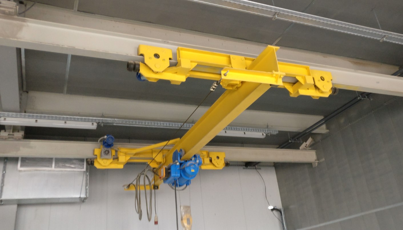
Table of Contents
The Core Physics: How Materials Stretch and Yield
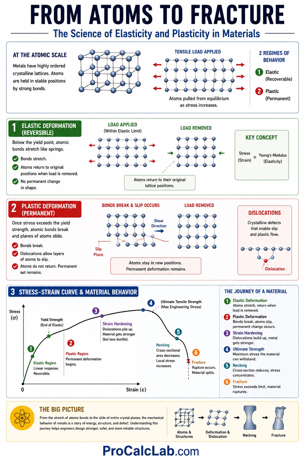
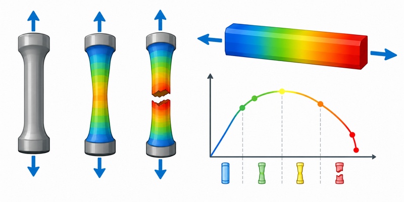
At the atomic scale, structural materials like steel, aluminum, and titanium are organized in highly ordered, crystalline structures called lattices. When you apply an external tensile load to a metal bar, you are physically pulling those atoms away from their stable equilibrium positions. This molecular battle is governed by 2 distinct regimes of physical behavior: elastic deformation and plastic deformation.
Elastic deformation is the initial, reversible stage of loading. As long as the applied stress remains below the yield point, the chemical bonds stretching between the atoms act like microscopic springs. When you remove the external tension, these atomic bonds pull the atoms back to their original lattice coordinates, restoring the original shape of the component. The ratio of applied stress to the resulting elastic strain is constant for any given material, a value known as the modulus of elasticity or Young’s modulus.
Once the applied load exceeds the yield strength of the material, the mechanical behavior shifts permanently into plastic deformation. At this stage, the external force is strong enough to break the atomic bonds, causing entire planes of atoms to slide past each other along slip planes. This movement is facilitated by crystalline defects called dislocations. When the load is removed, the atoms do not return to their starting positions. The component retains a permanent set, permanently altered in its physical dimensions.
If you continue to increase the tension past the yield point, the material will undergo strain hardening, where the microscopic dislocations pile up against grain boundaries, making the metal temporarily stronger but more brittle. This progression continues until the stress reaches the ultimate tensile strength of the material, which is the maximum engineering stress the material can sustain. Beyond this point, the material begins to neck, forming a localized narrow zone where the cross-sectional area decreases rapidly. The local stress inside this necked region skyrockets until the material reaches its rupture threshold, resulting in a physical split.
When studying these mechanics, we must distinguish between engineering stress and true stress. Engineering stress is calculated using the original, undeformed cross-sectional area of the part. In reality, as a bar stretches, its diameter must shrink due to a physical relationship defined by Poisson’s ratio. True stress is calculated using the actual, instantaneous cross-sectional area at any given moment. During the necking phase, the true stress increases continuously right up to the point of rupture, even though the calculated engineering stress appears to drop.
The Mathematics of Stress, Strain, and Stiffness
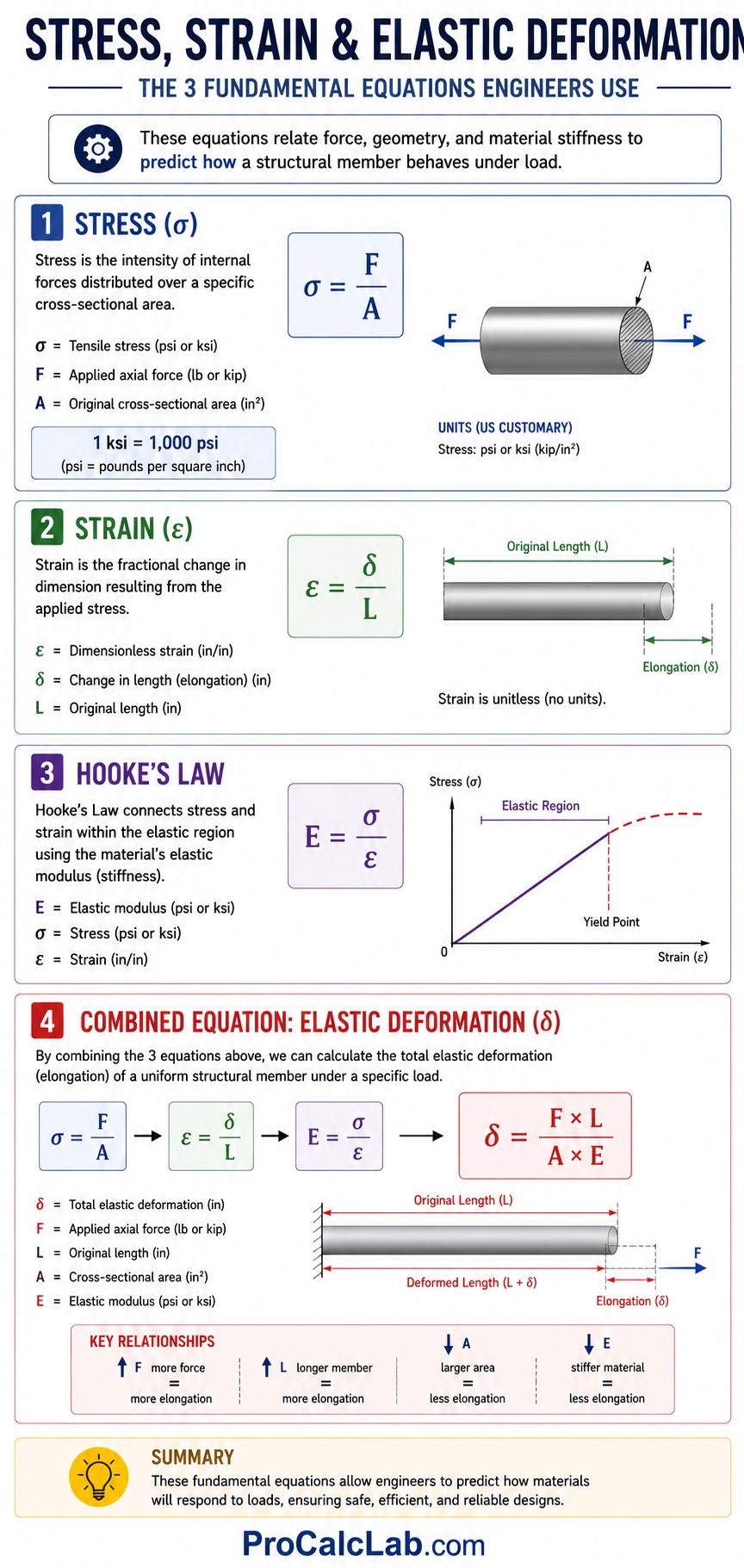
To quantify these physical changes, engineers rely on 3 fundamental equations that relate force, geometry, and material stiffness.
The 1st equation defines mechanical stress, which is the intensity of internal forces distributed over a specific cross-sectional area.
Stress is represented by the Greek letter sigma, and is calculated as follows:
σ = F / A
Where σ represents the tensile stress, F is the applied axial force, and A is the original cross-sectional area of the component. In the United States, stress is commonly expressed in pounds per square inch or kilopounds per square inch, where 1 kilopound per square inch, or ksi, equals 1,000 pounds per square inch.
The 2nd equation defines strain, which is the fractional change in dimension resulting from the applied stress. Strain is represented by the Greek letter epsilon, and is calculated as follows:
ε = δ / L
Where ε represents the dimensionless strain, δ is the total change in length or elongation, and L is the original length of the component.
The 3rd equation is Hooke’s Law, which connects stress and strain within the elastic region using the material’s elastic modulus, represented by the letter E:
E = σ / ε
By algebraic substitution, we can combine these 3 relations into a single formula to calculate the exact total elastic deformation of a uniform structural member under a specific load:
δ = F × L / (A × E)
This combined equation shows that elongation is directly proportional to both the applied force and the original length, but inversely proportional to the cross-sectional area and the stiffness of the material itself.
Step-by-Step Engineering Calculation
Let us apply these formulas to a real-world design scenario. Imagine you are designing a structural steel suspension rod to support a heavy industrial floor mezzanine inside a warehouse. The design specifications demand that the rod must support a continuous static load of 62,000 pounds. The length of the hanger rod is exactly 180 inches. For this application, you are evaluating a solid cylindrical rod made of ASTM A36 structural steel. This specific grade of steel has a yield strength of 36,000 pounds per square inch and a modulus of elasticity of 29,000,000 pounds per square inch. Your design goals are to determine the minimum rod diameter to achieve a target safety factor of 1.5 against yielding, and then calculate the total elongation of the rod under full load.
Step 1: Determine the allowable design stress
To ensure the rod operates safely inside its elastic limit, we must apply our safety factor to the yield strength of the steel. The allowable stress equals the yield strength divided by our safety factor of 1.5:
σallowable = 36,000 / 1.5 = 24,000 pounds per square inch
This calculation indicates that the maximum tension in our hanger rod must not exceed 24,000 pounds per square inch under the full 62,000-pound load.
Step 2: Calculate the required cross-sectional area
Using our stress equation, we rearrange the variables to solve for the minimum required area, A:
A = F / σallowable
A = 62,000 / 24,000 = 2.583 square inches
The solid steel rod must have a minimum cross-sectional area of 2.583 square inches to stay within our allowable stress limit.
Step 3: Calculate the required rod diameter
The cross-sectional area of a solid circular rod is defined by the geometry of a circle. We solve for the diameter, d, using the constant value of pi, which we will approximate as 3.14159:
A = 3.14159 × d2 / 4
Rearranging the equation to solve for d:
d = √(4 × A / 3.14159)
d = √(4 × 2.583 / 3.14159)
d = √(10.332 / 3.14159)
d = √(3.289)
d = 1.814 inches
From a practical standpoint, steel rods are sold in standard fraction increments. To maintain our safety factor, we must round up to the nearest commercial size, which is a 1.875-inch diameter rod. Let us recalculate the actual cross-sectional area using this real-world dimension:
Aactual = 3.14159 × 1.8752 / 4 = 3.14159 × 3.516 / 4 = 2.761 square inches
With this actual area, our real working stress drops to:
σactual = 62,000 / 2.761 = 22,456 pounds per square inch
This yields an actual safety factor against yielding of:
Safety Factor = 36,000 / 22,456 = 1.60
Step 4: Calculate the total elastic elongation under load
Now, we can calculate how much this 180-inch rod will physically stretch when the 62,000-pound load is applied. We plug our actual working parameters into our combined deformation equation:
δ = F × L / (Aactual × E)
δ = 62,000 × 180 / (2.761 × 29,000,000)
δ = 11,160,000 / 80,069,000
δ = 0.139 inches
Under a tension of 62,000 pounds, our 1.875-inch diameter structural rod will stretch by 0.139 inches, which is slightly over 1/8 of an inch. This level of elongation is perfectly acceptable and falls well within normal structural building design tolerances.
Material Properties and Strength Comparison
To design components that resist deformation and rupture, you must select the correct material. Different alloys exhibit radically different strength-to-weight ratios and stiffness values. The following 3 tables compare the critical mechanical properties of 4 common engineering metals. Table 1 outlines yield and ultimate strength in Imperial units. Table 2 details the same strength metrics in Metric units. Table 3 lists the elastic modulus for both unit systems, illustrating the comparative stiffness of each metal class.
Table 1: Structural Metal Strengths – Imperial Units
| Metal Alloy Name | Yield Strength in ksi | Ultimate Strength in ksi |
|---|---|---|
| ASTM A36 Structural Steel | 36 | 58 |
| 6061-T6 Aluminum Alloy | 40 | 45 |
| AISI 4130 Chromoly Steel | 63 | 97 |
| Titanium Grade 5 | 128 | 138 |
Table 2: Structural Metal Strengths – Metric Units
| Metal Alloy Name | Yield Strength in MPa | Ultimate Strength in MPa |
|---|---|---|
| ASTM A36 Structural Steel | 250 | 400 |
| 6061-T6 Aluminum Alloy | 276 | 310 |
| AISI 4130 Chromoly Steel | 435 | 670 |
| Titanium Grade 5 | 880 | 950 |
Table 3: Material Stiffness – Elastic Modulus
| Metal Alloy Name | Modulus in Mpsi | Modulus in GPa |
|---|---|---|
| ASTM A36 Structural Steel | 29 | 200 |
| AISI 4130 Chromoly Steel | 29 | 200 |
| Titanium Grade 5 | 16.5 | 114 |
| 6061-T6 Aluminum Alloy | 10 | 69 |
A close inspection of Table 3 reveals an essential engineering truth: alloy composition and heat treatment do not significantly affect a material’s elastic stiffness. For instance, AISI 4130 Chromoly steel is nearly 2 times stronger than A36 structural steel, yet they share the exact same elastic modulus of 29,000,000 pounds per square inch. This means that if you replace an A36 steel beam with a high-strength chromoly beam of the exact same dimensions, it will sag by the exact same amount under an identical load. The chromoly beam simply has a much higher yield point, meaning it can handle far greater loads before taking on a permanent bend.
Simulating Stress Concentrations and Geometrical Realities
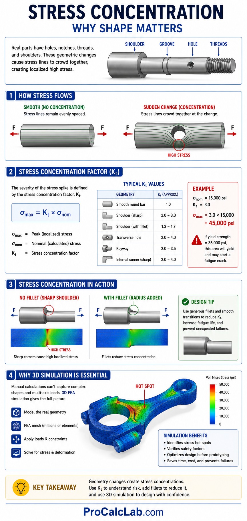
Our walkthrough calculation assumed a perfectly uniform, straight cylindrical rod. In the real world, mechanical components are rarely this simple. Real parts feature mounting holes, retaining ring grooves, notches, threads, and sharp shoulders where the diameter of a shaft shifts down to fit a bearing. These geometric changes introduce a major physical phenomenon known as stress concentration.
When tensile forces flow through a component, the internal lines of stress act like moving water. If the cross-section changes smoothly, the stress lines remain evenly spaced. However, if the stress lines encounter a sudden barrier, such as a sharp internal corner or a transverse hole, they are forced to crowd together to pass the obstacle. This localized crowding results in a massive spike in stress right at the boundary of the geometric change.
The severity of this spike is quantified by the stress concentration factor, represented by the letters Kt. The localized peak stress is calculated by multiplying the nominal calculated stress by this Kt factor. For a sharp 90-degree internal corner, Kt can easily range from 2 to 4. This means a component with a nominal calculated stress of 15,000 pounds per square inch might actually experience a localized stress of 45,000 pounds per square inch at a sharp fillet corner. If the yield strength of the material is 36,000 pounds per square inch, that localized zone will undergo permanent plastic deformation, eventually initiating a fatigue crack that will propagate through the part until it ruptures.
Calculating these stress concentrations manually for complex, multi-axis parts is nearly impossible. This is where 3D strength and deformation simulation becomes an indispensable tool. A 3D simulator utilizes Finite Element Analysis to divide a solid CAD model into 1,000,000s of tiny tetrahedral blocks. The simulator calculates the force balance, strain, and stress across every individual block, mapping out the precise locations of stress concentrations. By color-coding the results, a simulator allows engineers to instantly identify localized hot spots where stress exceeds the yield point or ultimate tensile strength, enabling them to modify geometries with generous fillets or transitions before physical prototyping begins.
Practical Engineering Challenges and Field Troubleshooting
In the field, designing a component to pass a simple static tensile test is only the 1st step. Real structural assemblies operate in harsh environments where other mechanical factors will quickly compromise your calculated safety margins.
The Threat of Mechanical Fatigue
Statistically, over 80% of all mechanical failures in operating machinery are caused by metal fatigue. Fatigue occurs when a component is subjected to repeated, cyclical loads rather than a single static load. Each time the load is applied and released, microscopic slips occur at stress concentration points. Over 1,000s or 1,000,000s of cycles, these slips coalesce into a microscopic crack. Once a crack forms, it acts as an ultra-sharp stress concentrator, propagating deeper into the material with each subsequent cycle. Eventually, the remaining solid cross-section of the part becomes too small to support the load, and the part undergoes a sudden, catastrophic brittle fracture, even if the nominal operating stress was always well below the material’s yield strength. To combat fatigue, engineers must design parts using fatigue limit values, which are significantly lower than the static yield strength.
Thermal Strain and Constrained Expansion
Another common field failure occurs when engineers forget to account for thermal expansion. Almost all structural metals expand when heated and contract when cooled, a relationship governed by the coefficient of thermal expansion. If a structural beam or pipe is welded rigidly between 2 immovable walls, any change in temperature will generate massive internal stresses. For example, if a steel beam is locked in place and heated by 50 degrees Fahrenheit, the restriction of its natural thermal expansion will generate 1,000s of pounds of internal compressive force, which can easily cause the beam to buckle. Designers must always incorporate expansion joints, slotted mounting holes, or flexible loops to allow materials to deform freely under thermal cycles.
Corrosion and Stress Corrosion Cracking
Environmental factors can accelerate material failure. When a high-strength metal is subjected to continuous tensile stress in a mildly corrosive environment, it can undergo stress corrosion cracking. This physical process allows cracks to grow at stress levels far below the normal threshold. Similarly, exposure to atomic hydrogen, which is often a byproduct of electroplating or corrosive chemical reactions, can cause hydrogen embrittlement. The tiny hydrogen atoms diffuse into the metal’s crystalline lattice, locking the dislocations in place and turning a ductile steel alloy into a brittle glass-like material that will rupture suddenly without any warning deformation.
Summary and Interactive Simulation Tools
Mastering the principles of material deformation is vital to creating safe, efficient structures and mechanical assemblies. By understanding how atomic bonds react to external tension, utilizing basic stress and strain equations, and accounting for the physical realities of stress concentrations, engineers can design components that handle extreme environmental forces without yielding or rupturing. Always remember that a safe static calculation is only the starting point; you must also design for fatigue, thermal expansion, and environmental factors to ensure long-term structural integrity.
Attempting to calculate the exact stress distribution, strain fields, and safety margins for a complex, 3D component with multiple holes, notches, or variable loads by hand is an exhausting, error-prone task. To bypass these limitations and visualize exactly how different materials and geometries respond to mechanical forces, utilize our interactive 3D strength and deformation simulator. By inputting your custom geometries, selecting from a database of real engineering alloys, and applying axial or torsional loads, you can instantly render high-fidelity color stress maps, evaluate local safety factors, and find the exact physical boundaries of structural failure in real-time.
Engineering References and Academic Literature
- Hibbeler, R. C. Mechanics of Materials. Pearson. This textbook is the definitive academic authority on the mechanics of stress, strain, elastic deformation, and beam deflection calculations.
- Pilkey, W. D., and Pilkey, D. F. Peterson’s Stress Concentration Factors. Wiley. The gold-standard engineering reference manual for analyzing Kt values across diverse geometrical features, shafts, and plates.
- Boyer, H. E. Atlas of Stress-Strain Curves. ASM International. A comprehensive compilation of physical material testing data, detailing tensile strength, yield limits, and plastic behavior for hundreds of metal alloys.

David Parry — Senior Engineering Analyst
Specializing in electronics and physics-based simulations with 20+ years of engineering experience. David ensures the mathematical and physical accuracy of the tools at ProCalcLab.