3D Power Emission of Antenna Architectures

Wireless networks run the modern world, yet the actual forces connecting our devices remain completely invisible. Every time a router boots up or a radio tower powers on, a complex three-dimensional web of electromagnetic energy bursts into the surrounding airspace. Understanding the precise shape of this energy cloud is the ultimate secret to building reliable networks. Field engineers, network architects, and hardware builders rely on spatial emission models to push signals through concrete walls, across massive agricultural fields, and up to orbiting satellites.

📊 This interactive visualization tool bridges the gap between complex physics and practical deployment. It translates abstract mathematical formulas into rendered three-dimensional objects. By manipulating frequencies and physical parameters, network builders can see exactly where a signal is going and, more importantly, where it is entirely absent. This guide breaks down the core mechanics of the simulator, explains the engineering behind the ten available architectures, and provides real-world math to guarantee successful hardware deployments.

Navigating the Spatial Simulator

The visualizer is built for speed and immediate feedback. It requires zero installation and runs complex phase calculations directly in the browser. The layout is divided into distinct operational zones designed for a seamless engineering workflow.

1. The top section features a horizontal array of ten selector buttons. Each button loads a completely different physical architecture into the rendering engine. Clicking a button instantly swaps the mathematical model and alters the variable parameter slider below to match the specific traits of the chosen hardware.
2. The central display area houses the interactive 3D canvas. This is a fully rotatable spatial playground. Clicking and dragging the mouse rotates the emission model, allowing an inspection of the energy lobes from any angle. Panning moves the camera side to side, and scrolling handles deep zooming. To maintain orientation, a static coordinate legend sits just below the canvas. The red line represents the horizontal X plane, the green line marks the vertical Y plane, and the blue line indicates the primary forward Z direction.
3. The control rows below the canvas handle the exact dimensional inputs. The frequency slider spans from the VHF bands at 100 MHz all the way up to the Wi-Fi and microwave bands at 6000 MHz. Adjusting this slider immediately calculates the new free-space wavelength. Because hardware size is permanently bound to wavelength, changing the frequency directly scales the physical dimensions reported in the results table.
4. The parameter slider is dynamic. Depending on the active profile, it might control the number of physical elements on a boom, the diameter of a metal dish, or the dielectric constant of a fiberglass circuit board. Moving this slider warps the 3D mesh in real time. Users can watch main beams grow razor-thin as gain increases or see side lobes erupt when a system is pushed past its optimal limits.
5. The results table serves as the final readout. It displays the wavelength in millimeters or centimeters, the overall physical footprint of the array, the peak forward gain in dBi, and the horizontal and vertical beamwidths in degrees. A final download button captures a crisp image of the current 3D state for easy inclusion in project documentation.

Decoding the Ten Core Architectures

Every specific job requires a specific shape of energy. A system designed to blast a narrow beam across a canyon will fail entirely if used to provide blanket Wi-Fi coverage in an office building. Here is the breakdown of the ten profiles and exactly where they belong in the field.

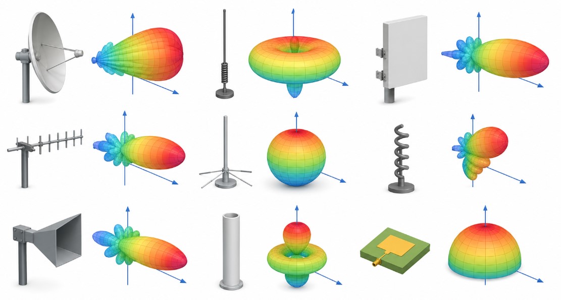
Isotropic Baseline

The isotropic radiator is a mathematical ghost. It does not exist in reality. It is a theoretical point in space that radiates power equally in every single conceivable direction, forming a flawless, smooth sphere. While impossible to manufacture, it is the fundamental measuring stick for the entire wireless industry.

When professionals say an array has a gain of 10 dBi, the “i” stands for isotropic. It means the physical hardware squishes and focuses the energy ten decibels stronger in one specific direction compared to that perfect, theoretical sphere. Selecting this profile in the tool provides the visual baseline that all other shapes are measured against.

Half-Wave Dipole

The dipole is the undisputed workhorse of global communications. Built from two identical conductive rods meeting in the center, its total length is cut to exactly one-half of the target wavelength. The spatial visualization reveals a shape exactly like a plump donut. The rod passes straight through the empty hole of the donut.

The strongest signal pushes out perpendicular to the metal. Pointing the end of the rod directly at a receiver guarantees a dropped connection because the ends radiate zero energy. When mounted vertically on a mast, the donut flattens out to cover the horizon, making it ideal for standard point-to-multipoint broadcasting. Playing with the parameter slider shows what happens when the wire is cut too long. The donut shatters into multiple erratic spikes, destroying the clean horizon coverage.

Grounded Monopole

The monopole cuts the dipole in half. It uses a single vertical rod measuring one-quarter wavelength, mounted over a flat metal surface or the steel roof of a vehicle. The metal surface acts as an electromagnetic mirror, tricking the radio waves into believing the lower half of the dipole still exists.

This design forces all the energy that would normally travel into the dirt to bounce up and combine with the upper hemisphere. The visual model shows a dome shape skimming the ground. This compression boosts the efficiency, pushing the standard gain to 5.15 dBi. It is the absolute standard for police cruisers, delivery trucks, and maritime vessels requiring omnidirectional range without carrying massive metal structures.

Yagi-Uda Array

When distance is the only goal, the Yagi-Uda array is the traditional answer. It features a long central boom loaded with multiple parallel rods. Only one rod connects to the radio. The rod behind it acts as a solid wall, reflecting energy forward. The numerous rods in front act like a magnifying glass, pulling the radio wave into a tight, focused beam.

The 3D canvas illustrates a long, aggressive teardrop shape pushing hard along the Z axis. Adjusting the slider to add more elements dramatically stretches this teardrop, increasing the gain. However, the visualization also reveals the fatal flaw of the Yagi. As the forward beam grows, small parasite lobes sprout out the back and sides. These side lobes absorb interference from nearby electronics, making careful aiming mandatory.

Microstrip Patch

Modern consumers despise ugly metal spikes sticking out of their devices. The patch antenna solves this by hiding the radiator inside the chassis. It consists of a flat copper square printed on a circuit board, backed by a solid copper ground plane. The dielectric material between the layers determines the efficiency.

The solid metal back completely blocks any rearward energy. The 3D model shows a wide, soft dome pointing straight out from the flat face. With a beamwidth hovering around 65 degrees, it perfectly covers a standard room or an outdoor plaza. Network engineers stack dozens of these tiny patches together inside plastic radomes to build the flat rectangular cell tower panels seen along highways.

Resonant Loop

The loop design bends a continuous wire into a closed circle or square. When the total perimeter length perfectly matches one full wavelength, the electrical currents align to shoot energy straight through the open center of the hoop. The spatial model looks like a thick barbell, pushing equal power to the front and the rear.

The true power of the loop lies on its sharp outer edges. The signal drops to an absolute zero along the rim. Radio trackers and signal hunters use this deep null to locate rogue transmitters. By spinning the loop until the target signal completely disappears, they can draw a laser-straight line on a map toward the source of the interference.

Axial Helical

Firing signals at drones, weather balloons, or satellites introduces a massive problem. When the flying object rolls or flips, its internal antenna flips too. If a vertical wave hits a horizontal receiver, the signal suffers a catastrophic 20 dB polarization loss. The helical design completely eliminates this risk.

By winding thick wire into a spring-like coil, the electromagnetic field is forced to spin like a corkscrew as it travels through space. The 3D model displays a long, forward-pointing cone. Because the wave is spinning, it successfully connects with the remote receiver regardless of how the flying object is oriented. Increasing the number of turns on the slider instantly narrows the cone and extends the reach.

Electromagnetic Horn

A horn resembles a heavy metal funnel. It transitions the high-pressure radio waves flowing inside a waveguide out into the open air without causing disruptive internal reflections. Because the walls are solid metal, no energy leaks to the sides or rear.

The visualizer shows an incredibly pristine, egg-shaped forward lobe. It lacks the messy parasitic spikes seen on a Yagi. This extreme purity makes the horn the ultimate laboratory tool. Engineers use them in anechoic chambers to calibrate other equipment, knowing the beam is mathematically perfect. In the field, they are used to feed microwave energy into larger reflector dishes.

Parabolic Reflector

The parabolic dish is the king of raw gain. It uses a curved metal bowl to catch scattered RF energy and bounce it into a single, intense focal point. A small feed unit sits at that focal point to collect the concentrated power. Conversely, during transmission, the feed blasts the bowl, which throws a massive, parallel wall of energy across miles of open space.

The 3D model reveals a terrifyingly sharp needle beam. At higher frequencies, the beamwidth shrinks to just 2 or 3 degrees. While the gain figures are staggering, frequently pushing past 30 dBi, the installation requires absolute mechanical perfection. A heavy wind gust twisting the mounting pole by just an inch can throw the needle beam completely off target, instantly severing a critical data link.

Collinear Array

When a town needs blanket coverage stretching out to the horizon, builders stack multiple dipoles vertically into a single long fiberglass tube. Phase-shifting coils placed between the segments ensure that all the energy waves push outward at the exact same fraction of a second.

This vertical stacking crushes the standard dipole donut flat. The spatial view shows a thin, razor-sharp disc that extends 360 degrees horizontally. It takes all the wasted energy that would normally shoot up into the clouds or down into the dirt and redirects it straight into the neighborhoods. Changing the parameter slider to increase the stage count crushes the disc even thinner, pushing the signal miles further down the road.

Reference Data for Field Deployments

Understanding the theoretical shape is only half the battle. Matching the physical properties to the operational environment guarantees a stable link. The tables below outline the expected performance envelopes and environmental resistance for common builds.

System Architecture	Average Field Gain dBi	Horizontal Coverage Angle	Primary Deployment Scenario
Quarter-Wave Monopole	2.15 to 5.15	360 Degrees Omnidirectional	Mobile fleet dispatch and handheld transceivers
Resonant Wire Loop	2 to 4	90 Degrees Bidirectional	Indoor attic installations and noise rejection
Microstrip Patch	6 to 9	60 to 80 Degrees Forward	Warehouse inventory tracking and Wi-Fi access
Multi-Element Yagi	9 to 15	30 to 50 Degrees Forward	Rural broadband links and telemetry bridging
Axial Helix Coil	10 to 14	40 to 60 Degrees Circular	Low Earth Orbit satellite passes and drone video
Parabolic Reflector	20 to 35	2 to 10 Degrees Forward	Mountain-top microwave backhaul trunks

Cable selection is just as critical as the radiator shape. All the gain generated by a perfect array can be destroyed by running the signal through cheap, lossy coaxial cable. The higher the frequency, the faster the cable absorbs the power.

Coaxial Cable Standard	Loss at 400 MHz per 100 feet	Loss at 2400 MHz per 100 feet	Best Use Case
RG-58 Thin Wire	6.5 dB	Over 20 dB Fatal Loss	Short 3-foot jumpers inside equipment racks
RG-8X Mini	4.2 dB	13.5 dB Severe Loss	Medium runs for VHF and UHF vehicle mounts
LMR-400 Low Loss	1.5 dB	6.8 dB Acceptable	Standard tower runs for cellular and WISP gear
LMR-600 Heavy Duty	1.0 dB	4.4 dB Excellent	Long commercial mast runs and high-power setups

System Integration and the Math of the Airwaves

Every successful wireless project relies on a mathematical proof called the link budget. This accounting system tracks every decibel of energy from the moment it leaves the transmitter board to the moment it hits the receiver chip. If the final number stays above the receiver sensitivity threshold, the data flows. If it drops below, the link dies.

The core equation calculates the received power level. It adds the starting power and the physical amplification of the hardware, then subtracts the brutal losses caused by cables and open air.

P_rx = P_tx – L_c + G_tx – L_fs + G_rx

In this architecture, P_rx is the final received power. P_tx is the radio output power. L_c represents the total loss of all coaxial cables and connectors. G_tx and G_rx are the directional gains provided by the structures on both ends. L_fs is the Free Space Path Loss, which is the natural spreading of energy as it travels across miles of atmosphere.

The path loss is the largest enemy in the equation. It is calculated based on the distance and the operating frequency. Higher frequencies scatter much faster than lower ones.

L_fs = 36.6 + 20log₁₀(Distance in Miles) + 20log₁₀(Frequency in MHz)

Real-World Deployment Scenario on a Texas Ranch

To demonstrate how this theory builds actual networks, consider an agricultural engineer setting up a soil moisture monitoring system on a massive Texas cattle ranch. The sensors are located in a valley exactly 4.5 miles away from the main ranch house. The engineer chooses the 915 MHz ISM band because it offers excellent penetration through light brush and does not require an FCC broadcast license.

The remote sensor node runs on solar power and outputs a tiny signal of 100 milliwatts. In the RF world, 100 milliwatts equals exactly +20 dBm. To maximize battery life, the engineer decides to build a custom Yagi-Uda array for the sensor node to blast that weak signal straight back to the house.

First, the physical dimensions must be calculated using the imperial speed of light. The speed of a radio wave is roughly 11.8 billion inches per second.

Wavelength = 11800000000 / 915000000 = 12.89 inches

Plugging 915 MHz into the 3D visualizer and selecting the Yagi profile reveals the required geometry. Setting the parameter slider to 7 elements produces a tight forward beam. The tool indicates a gain of 11.6 dBi for this setup. The results table also shows that the main boom holding the 7 elements will be roughly 18 inches long. The engineer cuts aluminum tubing to the precise lengths dictated by the wavelength math and mounts the array on a 10-foot wooden pole, aiming it directly at the ranch house.

At the ranch house, the receiver sits on a desk. A 50-foot run of high-quality LMR-400 coaxial cable goes up to the roof. The engineer installs a rugged collinear array on the roof to provide 360-degree coverage, allowing future sensors to be added in any direction. The visualizer shows a 4-stage collinear provides about 8.5 dBi of gain. The cable specs show that 50 feet of LMR-400 at 915 MHz will lose about 2 dB of power.

Now, the engineer runs the Free Space Path Loss math for a 4.5-mile journey at 915 MHz.

L_fs = 36.6 + 20log₁₀(4.5) + 20log₁₀(915) = 108.9 dB of atmospheric loss

With all the environmental and hardware data collected, the full link budget determines if the project succeeds.

P_rx = 20 (Radio) + 11.6 (Yagi) – 108.9 (Air Loss) + 8.5 (Collinear) – 2 (Cable) = -70.8 dBm

The modern LoRa receiver chip on the desk requires a minimum signal of -120 dBm to read the data. A final resting power of -70.8 dBm means the link has a massive 49 dB safety margin. The rancher will receive uninterrupted soil data even during heavy Texas rainstorms, all because the spatial emission shapes were correctly matched to the terrain.

Advanced Installation Mechanics

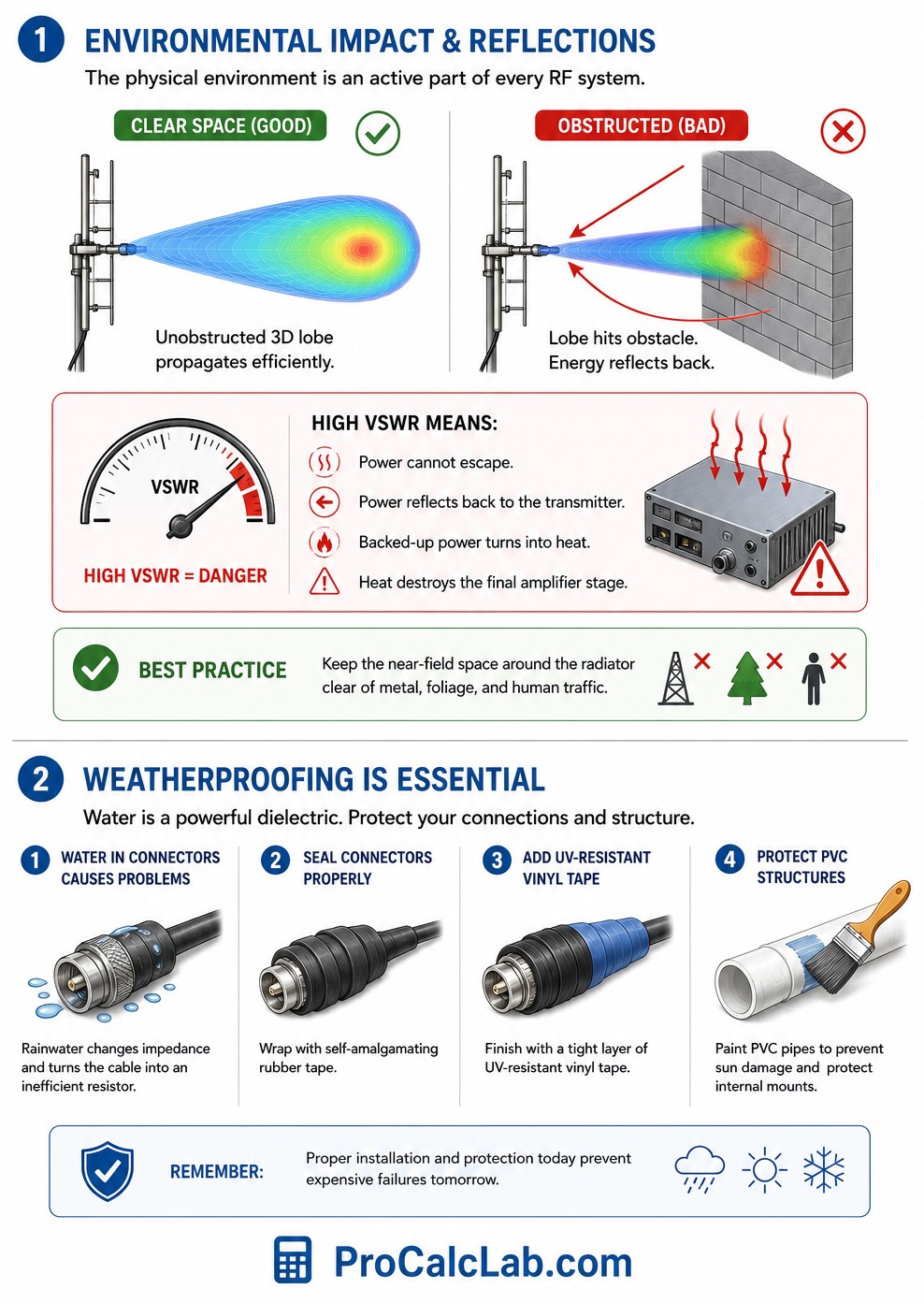
Deploying hardware outside of a controlled simulation introduces severe environmental variables. The physical environment acts as an active component in every RF circuit. When a metallic structure is mounted too close to a brick wall or a steel roof, the invisible 3D lobe slams into the obstacle. A portion of the wave absorbs into the masonry, but a massive percentage bounces directly back into the feed point.

📉 This backward reflection creates a Voltage Standing Wave Ratio error. High VSWR means the power cannot escape the metal. Instead, it backs up into the transmitter circuit as pure heat, eventually destroying the final amplifier stage. Builders must ensure that the immediate near-field space around a radiator remains entirely clear of conductive materials, heavy foliage, and human traffic.

Weatherproofing is the final mandatory step for any long-term deployment. Water acts as a powerful dielectric sink. If rainwater seeps into a coaxial connection, it drastically alters the impedance, turning the cable itself into a crude, inefficient resistor. Professionals wrap every outdoor connector in self-amalgamating rubber tape followed by a tight layer of UV-resistant vinyl tape. Additionally, any structural pipes made of PVC must be painted to prevent the sun from turning the plastic brittle and shattering the internal wire mounts.

Essential Technical Resources

Mastering the invisible geometry of the airwaves is a continuous journey. To dig deeper into the raw physics, fabrication techniques, and advanced array tuning, professionals rely on these established industry texts.

• The ARRL Antenna Book. Published by the American Radio Relay League. This is the absolute bible for hands-on builders. It contains thousands of pages of imperial cut charts, wire sizing rules, and practical fabrication advice for backyard and commercial towers alike.
• Antenna Theory and Design by Warren Stutzman and Gary Thiele. A cornerstone university text that strips away the mystery of array scaling and thoroughly explains the calculus behind pattern formation and side lobe suppression.
• Practical Antenna Handbook by Joseph Carr. An exceptional guide aimed directly at field technicians. It heavily focuses on matching networks, VSWR troubleshooting, and the actual mechanical construction of high-frequency hardware.
• Phased Array Antenna Handbook by Robert Mailloux. For those pushing into advanced Wi-Fi 6E, 5G cellular, and radar networks, this book breaks down how manipulating electrical timing can electronically steer a beam without using any moving mechanical parts.