3D Visualization in Mechanical Design

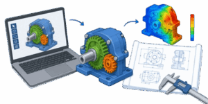
Standing on a bustling shop floor, watching a rigging crew attempt to force a 500-ton steel bridge crane into a space already occupied by a reinforced concrete pylon, represents the ultimate failure of spatial planning. In the era of traditional 2-dimensional drafting, a mechanical engineer had to hold 3 highly complex orthographic views in their head simultaneously. They had to mentally project top, front, and side elevations to hunt for invisible physical interferences. Mistakes were inevitable, and those mistakes cost millions of dollars in field rework.

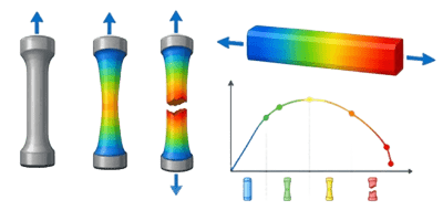
🧱 Modern 3-dimensional visualization has completely eliminated the guesswork from mechanical and civil engineering. Today, we do not simply draw lines on a digital page. We construct mathematically perfect virtual twins of our machinery before a single piece of steel is ever cut. 3-dimensional visualization serves as the foundational truth for kinematic testing, finite element analysis, and automated manufacturing pipelines.

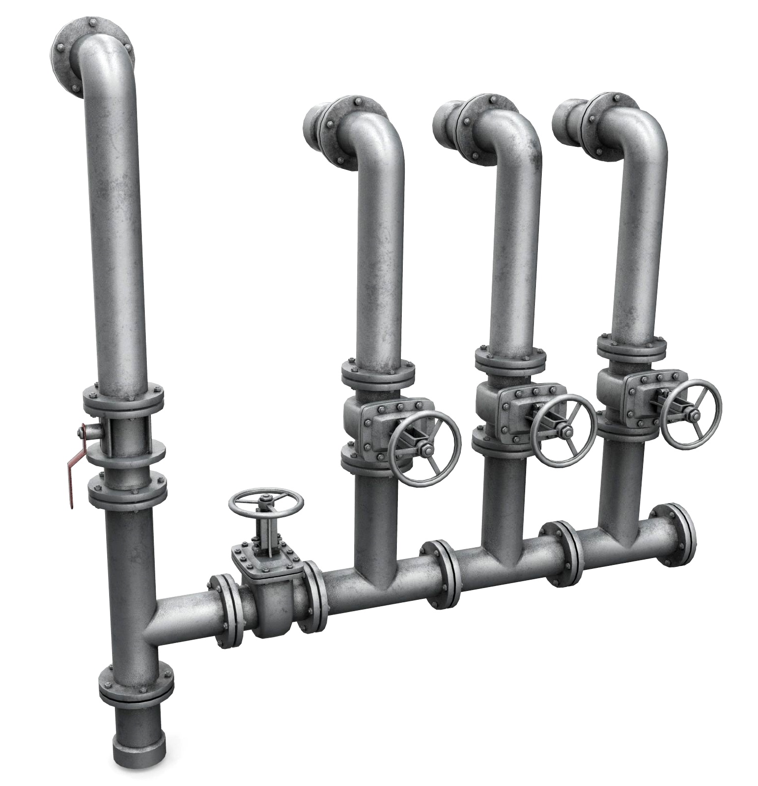
However, treating a 3-dimensional model as just a pretty picture is a severe operational error. These models are complex databases of geometric matrices, material densities, and parametric relationships. Understanding how software renders virtual space, how to extract usable mathematical data from these models, and how to troubleshoot inevitable rendering crashes is essential for any modern designer. This comprehensive guide breaks down the core mechanics of virtual space, details the math behind rendering loads, and provides professional strategies for managing massive digital assemblies.

The Physics of Virtual Space: Coordinate Systems and Degrees of Freedom

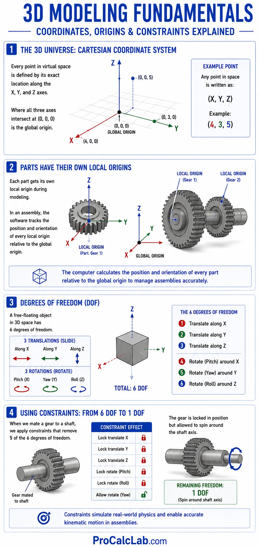
Before a computer can display a 3-dimensional object, it must establish a universe for that object to exist within. This universe is defined by the Cartesian coordinate system. Every single point in virtual space is tracked using an exact location along the X, Y, and Z axes. The point where all 3 axes intersect at exactly 0 is called the global origin.

⚙ When you model a mechanical part, such as a cast iron gear, the software assigns that specific part its own local origin. As you assemble multiple gears into a gearbox, the software calculates the distance and orientation of every local origin relative to the global origin. This is how the computer tracks distinct components without merging them into a single lump of digital clay.

In mechanical engineering, we use assembly constraints to simulate real-world physics. A free-floating object in a 3-dimensional universe possesses exactly 6 degrees of freedom. It can translate, or slide, along the X, Y, and Z axes. It can also rotate, or pitch, yaw, and roll, around those same 3 axes. When we mate a gear to a steel shaft, we apply geometric rules that strip away 5 of those degrees of freedom. We lock the translation along all 3 axes, and we lock the rotation along 2 axes. We leave exactly 1 degree of freedom open, which allows the gear to spin concentrically around the shaft. This mathematical lockdown is what allows engineers to simulate complex kinematic motion accurately.

Boundary Representation versus Tessellation

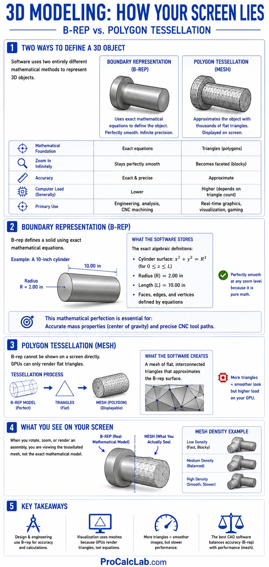
Software displays 3-dimensional objects using 2 entirely distinct mathematical methods. You must understand the difference between Boundary Representation and Polygon Tessellation to avoid crippling your computer hardware.

When you design a mechanical part in professional engineering software, the program uses Boundary Representation, commonly known as B-rep. B-rep defines a solid object using exact mathematical equations. If you draw a 10-inch cylinder, the software does not draw thousands of tiny flat lines to make a circle. Instead, it stores the exact algebraic equation for a cylinder, bounded by a specified radius and extrusion length. B-rep is perfectly smooth at an infinite zoom level because it is pure math. This perfection is necessary for extracting exact center of gravity data and calculating precise tool paths for computer numeric control milling machines.

💻 The problem is that graphic processing units cannot display pure algebraic equations on a monitor in real-time. Graphic cards are built to render flat triangles. Therefore, the software must run a background process called tessellation. Tessellation takes the mathematically perfect B-rep model and wraps it in a mesh of flat, interconnected triangles. This is the polygon mesh.

When you rotate an assembly on your screen, you are not actually looking at the exact mathematical model. You are looking at the tessellated mesh. The denser the mesh, the smoother the object looks, but the harder your graphic card has to work to calculate the light reflecting off every single triangle.

Dynamic Parametric Extraction and Field Tools

From a practical standpoint, a 3-dimensional model is only as useful as the metadata you can extract from it. Modern models are parametric, meaning their geometry is driven by variables rather than static lines. If you change a single dimensional variable, the entire model updates automatically, recalculating volume, mass, and surface area in milliseconds.

This dynamic data extraction bridges the gap between the engineering department and field operations. Instead of waiting weeks for a drafting team to manually revise 2-dimensional prints, project managers rely on dynamic visualization engines to generate instant takeoffs for clients. For instance, when securing commercial or residential perimeters, contractors utilize our custom 3-dimensional gate and fence estimator to instantly visualize property lines. The visualization engine automatically reads the virtual terrain, adjusts post heights for changing elevations, and calculates exact structural steel weight and infill surface area requirements directly from the spatial data.

This automated extraction eliminates human mathematical error. The visualization engine pulls the exact bounding box dimensions from the virtual parts, queries the assigned material density, and outputs a flawless bill of materials that procurement teams can order from immediately.

The Mathematics of System Resource Allocation

A common mistake during calculations is severely underestimating how much random access memory a highly detailed visualization requires. When junior designers model unnecessary microscopic details, they crash their workstations. To prevent hardware failure, engineers must calculate the graphic payload of their assemblies.

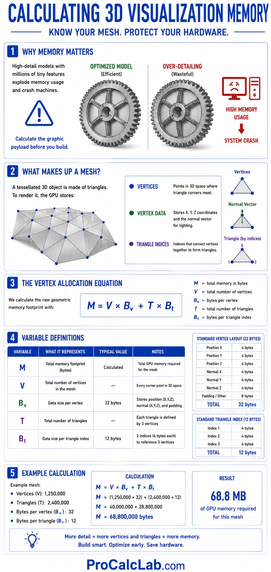
📊 The memory footprint of a tessellated 3-dimensional object is determined by its vertex count. A vertex is a single point in 3-dimensional space where the corners of triangles meet. To render an object, the graphic card must store the X, Y, and Z coordinates of every vertex. It must also store the normal vector, which tells the software which direction the surface is facing so it can calculate lighting shadows. Finally, it must store an index list that connects the vertices together to form the actual triangles.

We calculate the raw geometric memory footprint using the following vertex allocation equation:

M = V × B_v + T × B_t

Where each variable represents the following data points:

• M represents the total memory footprint in bytes.
• V represents the total number of vertices in the mesh.
• B_v represents the data size per vertex. A standard vertex requires 32 bytes to store its physical coordinates and lighting vectors.
• T represents the total number of triangles.
• B_t represents the data size per triangle index. A standard index requires 12 bytes to map its 3 connecting points.

Step-by-Step Graphic Load Calculation

Let us walk through a practical scenario. You are importing a highly detailed 3-dimensional scan of a V8 engine block into your assembly. The vendor provided a mesh containing exactly 2500000 vertices and 5000000 triangles. We must determine if this single component will exceed the available video memory on a standard engineering laptop.

Step 1: Calculate Vertex Memory

Multiply the total vertices by the standard 32-byte data requirement.

Vertex Memory = 2500000 × 32 = 80000000 bytes.

Step 2: Calculate Triangle Index Memory

Multiply the total triangles by the standard 12-byte index requirement.

Index Memory = 5000000 × 12 = 60000000 bytes.

Step 3: Calculate Total Raw Footprint

Add the vertex memory and index memory together.

Total M = 80000000 + 60000000 = 140000000 bytes.

Step 4: Convert to Megabytes

To convert bytes to megabytes, we divide by 1048576, which is the exact byte count in 1 true megabyte.

140000000 / 1048576 = 133.51 Megabytes.

This calculation proves that the raw geometry alone requires over 133 megabytes of continuous video memory. Once you add high-resolution material textures, anti-aliasing filters, and ambient occlusion shadows, this single engine block will consume nearly 500 megabytes of memory. If you place 10 of these engine blocks into a factory floor layout, you will instantly exhaust a standard graphic card, resulting in severe frame rate drops or a complete software crash.

Engineering Data Tables for Visualization Management

Managing digital performance requires strict adherence to industry standards regarding file types and polygon budgets. The tables below provide the baseline metrics used by professional engineering departments to maintain stable 3-dimensional environments.

Table 1: Polygon Mesh Resource Consumption

Visualization Application Type	Optimal Triangle Limit	Hardware Requirement Profile
Interactive Web Configurators	Under 50000 triangles	Lightweight. Renders smoothly on mobile processors.
Standard Component Design	100000 to 500000 triangles	Moderate. Requires a dedicated entry-level graphic card.
Full Vehicle Assembly Layout	5000000 to 10000000 triangles	Heavy. Demands a professional workstation graphic processing unit.
Photorealistic Marketing Renders	Over 20000000 triangles	Extreme. Requires server farm rendering clusters or prolonged calculation times.

Table 2: Common Spatial Data Formats

File Extension Format	Underlying Geometry Type	Primary Engineering Use Case
STEP	Boundary Representation Math	The gold standard for transferring exact solid models between different software brands.
IGES	Surface Representation	Used heavily in aerospace for defining complex curved outer molds without solid volume.
STL	Tessellated Polygon Mesh	Strictly used for 3-dimensional printing. Contains zero parametric math data.

Practical Troubleshooting in Virtual Environments

Even with pristine mathematical calculations, 3-dimensional modeling software is prone to visual glitches and kinematic errors. In the field, we often see entire engineering teams paralyzed by software bugs that are entirely preventable if you understand the underlying rendering mechanics. Below are the primary failure points and how to fix them.

Unsuppressed Cosmetic Hardware

✍ The number 1 cause of massive assembly failure is the inclusion of literal screw threads. When junior engineers download a fastener model from a supplier, the model often features physically cut helical threads. A single 0.5-inch bolt with true helical threads can easily contain 150000 triangles. If an engineer patterns that bolt 500 times across a structural steel frame, they inadvertently inject 75000000 triangles into the assembly.

The entire workstation will freeze. To prevent this, professional drafting standards dictate that all fasteners must use cosmetic threads. A cosmetic thread is simply a smooth cylinder wrapped in a 2-dimensional picture of a thread. The software recognizes it as a threaded hole for manufacturing drawings, but the graphic card only has to render a lightweight cylinder consisting of roughly 200 triangles. Always suppress physical helical cuts before placing hardware into a master assembly.

Z-Fighting and Coplanar Interference

✍ Have you ever looked at a 3-dimensional model and seen 2 surfaces violently flickering back and forth in a rapid, jagged pattern? This visual error is called Z-fighting. It occurs when 2 distinct solid bodies share the exact same mathematical plane in space. Because both surfaces are precisely equal in their distance from the digital camera, the graphic processor cannot decide which one should be drawn in front. It rapidly alternates between the 2, causing the flickering.

This happens frequently when a steel plate is mated flush against a concrete floor, and both parts are drawn without any clearance tolerance. To solve Z-fighting, you must introduce a microscopic physical offset. Moving the steel plate upward by just 0.001 inches resolves the mathematical tie, instantly curing the visual flickering without impacting the overall dimensional accuracy of the manufacturing blueprints.

Inverted Surface Normals

✍ Occasionally, you will import a part from a supplier and find that half of the surfaces appear to be completely invisible, allowing you to see inside the solid body. This happens due to inverted surface normals. Every polygon triangle has a front side and a back side. To save memory, rendering engines use a technique called backface culling, which tells the computer to completely ignore the back side of a polygon and render it invisible.

During file translations, the mathematical vector that defines the front of the triangle can accidentally get flipped, pointing inward toward the center of the part instead of outward toward the camera. The software assumes you are looking at the back of the polygon and renders it invisible. To fix this, you must open the mesh editing tools and use the recalculate normals command. This forces the software to analyze the solid volume and flip all vectors outward, restoring the visible surface of the part.

Gimbal Lock in Kinematic Articulation

✍ When simulating complex robotic arms or multi-axis machining centers, engineers rely on Euler angles to define rotation along the X, Y, and Z axes. However, a major mathematical flaw exists within the Euler system known as Gimbal lock. If you rotate a robotic arm such that 2 of its rotational axes perfectly align with one another, the system loses a dimension of space. You effectively lose 1 degree of freedom, and the simulation will act erratically, snapping the arm into unnatural positions.

To bypass Gimbal lock in advanced kinematic simulations, software developers abandon 3-axis Euler angles entirely and switch the calculation engine to Quaternions. A Quaternion is a highly complex 4-dimensional mathematical system that calculates rotation based on an arbitrary vector and an angle. While mathematically dense, Quaternions never suffer from axis alignment locking, ensuring that multi-joint robotic simulations move smoothly through all possible ranges of motion.

Final Design Considerations

The transition from flat 2-dimensional lines to dynamic 3-dimensional environments represents the greatest leap in engineering capability since the industrial revolution. By building exact digital twins, we eliminate physical prototyping costs, prevent catastrophic structural interferences, and automate the generation of perfectly accurate bills of materials.

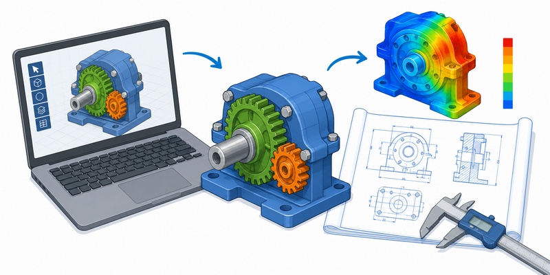
However, commanding this technology requires discipline. You must respect the hardware limits of your graphic processors by managing your polygon mesh counts. You must enforce strict parametric modeling practices so your assemblies update predictably, and you must ruthlessly suppress unnecessary geometric details to keep your master layouts lightweight and responsive. By mastering the mathematical mechanics of virtual space, you ensure that what you see on the screen translates flawlessly to the concrete reality of the job site.

Literature

• Foley, James D., et al. Computer Graphics: Principles and Practice. Addison-Wesley Professional. The definitive textbook detailing the mathematical algorithms behind polygon tessellation, coordinate transformations, and rendering pipelines.
• Shih, Randy H. Parametric Modeling with Autodesk Inventor. SDC Publications. A practical guide outlining the application of assembly constraints, degrees of freedom, and top-down skeletal modeling techniques in mechanical design.
• Zeid, Ibrahim. Mastering CAD/CAM. McGraw-Hill Education. An exhaustive technical reference covering boundary representation mathematics, kinematic articulation, and digital manufacturing workflows.