| Interval | - |
| Area S | 0.000 |
Calculating the geometric space enclosed by various mathematical lines is a fundamental task in practical computation. This process finds extensive application in modern digital design, structural loading estimation, material optimization, and statistical forecasting. Automated computation eliminates the traditional burden of manual integration, providing instant visual feedback alongside highly accurate numerical results. This guide serves as a comprehensive manual for operating the interactive workspace, understanding the core geometric principles, and interpreting the real-time data displayed on the screen.


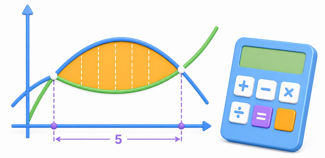
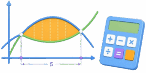
In standard geometry, determining space is restricted to regular polygons with straight edges. When boundaries involve curves, classical formulas fail. Calculus solves this by utilizing the definite integral, which continuously sums infinitely small vertical segments across a specified interval. The interactive solver automates this exact process. It tracks the behavior of lines on a coordinate grid, locates their intersections, establishes boundaries, and outputs the exact space enclosed by the curves without requiring any manual entry of antiderivatives.
Table of Contents
Interface Navigation and the 3 Operational Modes
The workspace is structured around 3 distinct tabs located at the top of the application container. Each tab corresponds to a specific mathematical scenario encountered in daily engineering or educational workflows. Switching between these tabs modifies the active control panel below the canvas, allowing customization of coefficients or formulas.
- Curve & X-Axis Mode: This control set focuses on a single quadratic curve defined by the equation f(x) = ax2 + bx + c. The calculation determines the space trapped between this specific line and the flat horizontal axis where y = 0. Users manually define the starting and ending vertical boundaries via independent interval inputs.
- Between Curves Mode: This automated routine handles 2 separate functions simultaneously. The system plots f(x) as an upper or lower boundary and g(x) as the opposing boundary. The software scans for intersection coordinates where f(x) = g(x). It uses these exact points as the natural calculation boundaries, removing the need for manual interval selection.
- Custom Formula Mode: Designed for advanced operations, this field accepts direct keyboard text input for f(x). It allows users to test custom polynomial behaviors beyond standard quadratic structures. The calculation requires manual input of the starting and ending coordinates to confine the integration space on the canvas.
Step-by-Step Guide to Adjusting Controls
Operating the solver involves adjusting interactive sliders and numerical input fields to shape the lines on the 2D canvas. The layout responds instantly to changes, updating both the visual fill color and the final numeric calculation table simultaneously.
- Step 1 requires choosing the calculation mode by clicking 1 of the 3 top tabs. For basic curve analysis, Tab 1 is ideal. For comparing 2 intersecting parabolas, Tab 2 offers automated tracking. For complex expressions, Tab 3 opens the text entry box.
- Step 2 involves manipulating the coefficient inputs. Each row features a twin-control setup: a horizontal range slider for rapid adjustments and a precise number input box for exact digital adjustments. Modifying Coeff. a scales the vertical steepness of f(x), while Coeff. b alters the slope, and Shift c moves the entire line up or down along the vertical axis.
- Step 3 defines the calculation span along the horizontal plane. In Manual and Custom modes, users shift the From x₁ slider to fix the left vertical boundary and the To x₂ slider to establish the right vertical boundary. The canvas instantly highlights the selected zone with a translucent light-blue fill color, utilizing the specific hex hue translated into a 30% alpha layer for optimal grid visibility.
- Step 4 concludes the interaction by reading the final data matrix or clicking the Update button to refresh the calculation. The Screenshot button triggers an immediate capture of the canvas rendering, which is useful for exporting visual data directly into external technical reports or study materials.
Mathematical Foundations Without Dense Theory
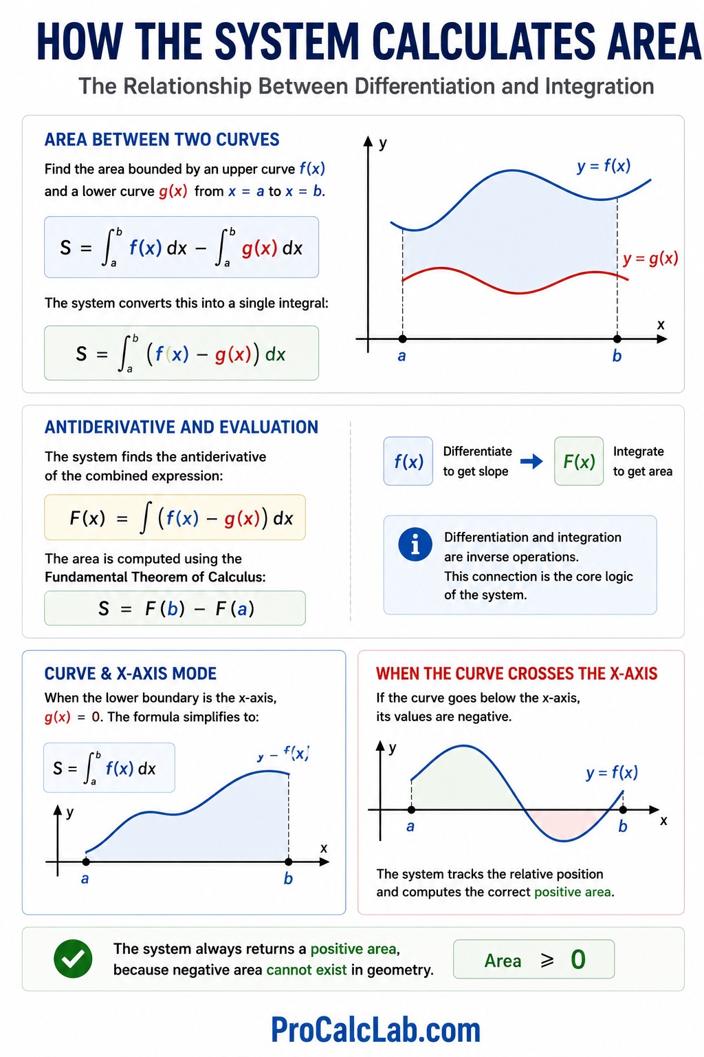
The core logic of the system relies on the relationship between differentiation and integration. To find the space bounded by an upper curve f(x) and a lower curve g(x) from a left boundary a to a right boundary b, the system computes the definite integral of their difference. This is represented by the formula:
S = ∫ab f(x) dx – ∫ab g(x) dx
The software converts this into a single operation:
S = ∫ab f(x) – g(x) dx
It determines the antiderivative function F(x) for the combined expression. The final area is computed by evaluating this antiderivative at the upper limit and subtracting its value at the lower limit, following the standard rule:
S = F(b) – F(a)
When working in Curve & X-Axis mode, g(x) is zero. The expression simplifies to the area underneath a single line. If a curve sinks below the horizontal axis, its coordinate values become negative. The solver handles this by tracking the relative position of the boundaries, ensuring that the final output for the space remains positive, as negative area cannot exist in physical geometry.
Comprehensive Reference Tables
The following tables provide reference data for verifying integration results, understanding control interactions, and resolving common visual setup issues on the canvas.
Table 1. Common Polynomial Functions and Their Antiderivatives
| Input Function Type f(x) | Antiderivative Form F(x) | Geometric Behavior on Grid |
|---|---|---|
| 0 | C | Flat horizontal line matching the X-axis |
| 5 | 5 * x + C | Horizontal baseline shifted 5 units up |
| x | x2 / 2 + C | Straight diagonal line at a 45-degree angle |
| x2 | x3 / 3 + C | Standard U-shaped symmetrical parabola |
| x3 | x4 / 4 + C | S-shaped cubic curve passing through the origin |
| 3 * x2 | x3 + C | Steepened parabola with accelerated vertical growth |
Table 2. UI Control Sliders and Their Graphic Impact
| Control Label | Mathematical Role | Visual Result on Canvas Display |
|---|---|---|
| Coeff. a | Quadratic multiplier | Controls width and direction of parabola opening |
| Coeff. b | Linear multiplier | Shifts the vertex diagonally across the grid |
| Shift c | Constant intercept | Moves the line vertically up or down |
| From x₁ | Lower integration limit | Moves the left boundary line of the shaded area |
| To x₂ | Upper integration limit | Moves the right boundary line of the shaded area |
Table 3. Troubleshooting Boundary Conditions and Errors
| Observed Issue | Root Mathematical Cause | Practical User Correction Steps |
|---|---|---|
| Area reads 0.000 | Limits x₁ and x₂ are equal | Adjust the sliders to separate the boundary lines |
| Area reads 0.000 | Curves do not intersect | Switch to Manual mode or adjust vertical shift c |
| Shaded area looks wrong | Incorrect formula syntax | Use explicit multipliers such as x * x instead of xx |
| Interval displays a dash | No real roots exist | Change coefficients to make the formulas cross paths |
Fully Solved Practical Example: Line and Parabola Intersection
✍ To demonstrate how the system processes data behind the scenes, consider a scenario involving 2 distinct lines. The upper boundary is a downward-sloping linear function: f(x) = 4 – x. The lower boundary is a standard upward-opening parabola shifted down: g(x) = x2 – 2. We need to find the total enclosed space between their intersection points.
First, the system determines the boundaries by finding where the lines cross. This requires setting f(x) = g(x), resulting in the equation: 4 – x = x2 – 2. Moving all terms to 1 side yields a standard quadratic equation: x2 + x – 6 = 0.
Solving this quadratic equation involves factoring the terms: 1 * x2 + 1 * x – 6 = 0. The factors are 3 and -2, because 3 * -2 = -6, and 3 – 2 = 1. This gives the rewritten form: x + 3 * x – 2 = 0. The roots of this equation define the integration limits: x₁ = -3 and x₂ = 2.
Next, the system confirms which function is higher on the interval from -3 to 2. Choosing a test value of 0 inside this range, f(0) = 4 – 0 = 4, and g(0) = 02 – 2 = -2. Since 4 is greater than -2, the straight line f(x) sits above the parabola g(x) throughout the highlighted zone.
Now, the system constructs the difference function for integration: f(x) – g(x) = 4 – x – x2 – 2 = 6 – x – x2. The next step involves calculating the antiderivative F(x) for this combined expression. The individual parts integrate as follows: the antiderivative of 6 is 6 * x, the antiderivative of -x is -x2 / 2, and the antiderivative of -x2 is -x3 / 3. Combining these results gives the total antiderivative function: F(x) = 6 * x – x2 / 2 – x3 / 3.
The solver evaluates this antiderivative at the upper limit x₂ = 2. Substituting 2 into the expression: F(2) = 6 * 2 – 22 / 2 – 23 / 3 = 12 – 4 / 2 – 8 / 3 = 12 – 2 – 2.67 = 7.33.
Then, the solver evaluates the antiderivative at the lower limit x₁ = -3. Substituting -3 into the expression: F(-3) = 6 * -3 – -32 / 2 – -33 / 3 = -18 – 9 / 2 – -27 / 3 = -18 – 4.5 + 9 = -13.5.
Finally, the system calculates the difference between the upper and lower evaluations to find the total area: S = F(2) – F(-3) = 7.33 – -13.5 = 7.33 + 13.5 = 20.83. The interactive canvas instantly displays 20.830 inside the green area result cell while rendering the corresponding shape on the grid.
Real-World Applications of Bounded Area Solvers
The mathematical process of finding the space between curves is not just an academic exercise. It is a vital tool used across multiple industries to optimize designs, predict behaviors, and analyze data efficiency.
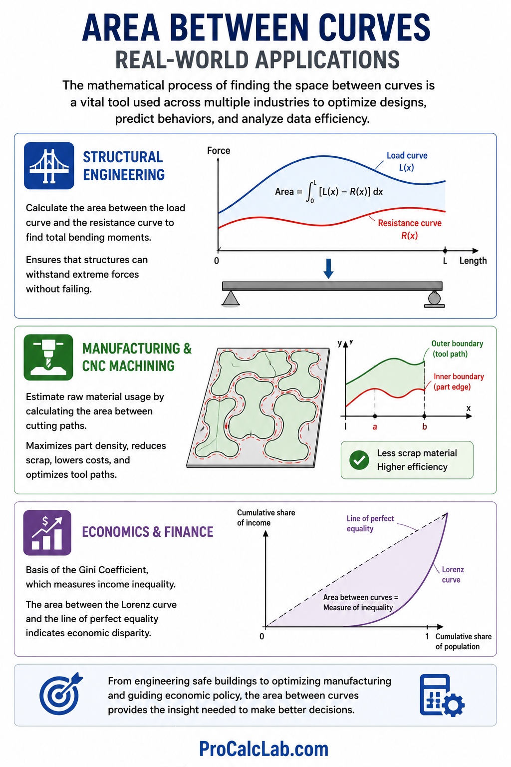
In structural engineering, calculating the area between curves helps determine the distribution of stress inside beams and columns. When a load is applied to a building component, the internal forces vary across its length. By integrating the difference between the load curve and the resistance curve, engineers calculate total bending moments, ensuring that structures can withstand extreme forces without failing.
In manufacturing and CNC machining, this methodology helps estimate raw material consumption. When cutting complex curved parts from flat metal sheets, tracking the space between the cutting paths allows software to maximize part density. This minimizes scrap material, reduces production costs, and optimizes tool paths for faster manufacturing cycles.
In economics and finance, this calculation forms the basis of the Gini Coefficient, which measures wealth distribution inequality within a population. Economists plot a curve representing perfect income equality against the actual Lorenz curve of a nation. The area trapped between these 2 lines indicates the level of economic disparity, serving as a guide for adjusting national fiscal policies.
Recommended Reference Books for Further Study
- Stewart, J. Calculus: Early Transcendentals. A globally recognized textbook offering clear explanations of definite integrals and practical applications of area calculations.
- Thomas, G. B., Weir, M. D., & Hass, J. Thomas’ Calculus. A comprehensive guide focusing on analytical geometry, integration techniques, and coordinate grid mathematics.
- Larson, R., & Edwards, B. H. Calculus. An engineering-focused textbook featuring detailed breakdowns of polynomial integration and visual area models.
- Strang, G. Calculus. An open-education classic from MIT that connects the theory of integration with practical computational workflows and numerical solvers.

Markus Fletcher — Structural Design Specialist
Expert in structural integrity, 3D modeling, and applied mathematics. Markus focuses on creating precise tools for construction professionals and DIY engineers.


